A Paradox of Blown Leads:
Rethinking Win Probability in Football
Authors:
Jonathan Pipping, Ph.D. Student, Wharton Sports Analytics and Business Initiative Research Team
Abraham J. Wyner, Faculty Co-Director, Wharton Sports Analytics and Business Initiative
Published: July 4, 2025
Introduction
Over the last 15 years, an explosion of publicly available NFL play-by-play data has made it possible to model the win probability of teams at any point in a game. Brian Burke published the first of these open-source models in 2014, and in the years since, they have become ubiquitous in sports media and game broadcasts. Even the most casual sports fans have probably seen a win probability graphic like Figure 1, which makes it possible to visualize the story of a game as the evolution of a single number.

Figure 1: ESPN’s win probability graphic for Super Bowl LVII between the Kansas City Chiefs and the Philadelphia Eagles. A link to the graphic is available here.
These graphics are easy to understand, and assuming they’re well-calibrated, they can be interpreted as the probability that a team will win based on the current state of the game. For example, with 1:56 left in the 2nd quarter of Super Bowl LVII, the Eagles led 21-14 and had just forced a 1st and 10 incompletion from QB Patrick Mahomes. After this play, ESPN Analytics estimated the Eagles’ win probability at 67%, meaning that we would expect the Eagles to win from this position about 2/3rds of the time.
As we know now, the Eagles did not go on to win, losing 38-35 on a last-second field goal. How might we interpret this result in the context of these win probability estimates? Most people, including professional analysts, might suggest that the Eagles blew the Super Bowl, since a team losing from a 67% estimated win probability should only happen 1/3rd of the time. Some might go even further, observing that the Eagles obtained a maximum win probability of 78.4% early in the 3rd quarter and call their defeat particularly extraordinary; after all, the model suggests we should only expect them to lose from this position about 21.6% of the time! While this may seem like an intuitive interpretation, it’s actually very wrong – but why?
First, let’s consider the general setting of a two-team game with no ties. In these games, there is guaranteed to be one winner who attains a win probability of 100% at the end of the game, exceeding all other possible win probabilities in the process. What does this mean for our discussion of the Eagles’ Super Bowl defeat, and losing teams in general? Having a maximal win probability below 100% implicitly guarantees that the team lost that game. This means that to properly analyze the significance of a blown lead, we can’t just use the maximal win probability obtained by a loser in a single game; we need to compare this maximum to the maximum win probabilities obtained by all other losing teams. What does this distribution really look like? We answer these question by designing a simulation study where we know the true win probability of both teams at every stage of the game.
Simulation Study
Setup
Deriving the win probability of a team at any point in a football game is a complex problem, but we make some simplifying assumptions to make a written derivation possible. First, we assume that each team has an equal number of possessions N , and that each possession ends with a touchdown or a punt. Next, we assume that the teams are equally-matched, and each has a 50% chance of scoring a touchdown on each possession. Finally, we assume that if the teams tie, the game goes to overtime and is decided by a fair coin flip.
With these assumptions, we can express the win probability of team A as the probability that they outscore team B plus the probability that they tie and win in overtime. Written mathematically, we have that

Then our scoring assumptions allow us to express the win probability for team A after possession t as
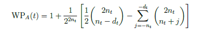
Procedure
With this closed-form expression in hand, we simulate 10,000 games between team A and team B, setting the number of possessions N = 10, 000 to emulate the near-continuous nature of win probability plots. We calculate the win probability of both teams after each possession, see who lost the game, and extract the maximum win probability they attained. The win probability trajectory of one of these losing teams is pictured in Figure 2, peaking at 98.5% before they eventually lost.

Figure 2: Win probability trajectory of the losing team in one of the simulated games. The blue dot denotes when they achieved their maximum win probability of 98.5%.
Results
Since we have the true maximum win probability of the losing team for each simulated game, we can plot the distribution of these values, which is shown in Figure 3. Since teams are evenly matched, this quantity ranges from 0.5 (the starting win probability) to 1.0. This distribution shows a clear downward trend, which aligns with our intuition that losing teams are less likely to attain higher win probabilities.

Figure 3: Distribution of the maximum win probabilities of the losing team. Since teams are evenly-matched, this ranges from 0.5 to 1.0 and decreases smoothly over this range. The mean of this distribution is 0.690, and its standard deviation is 0.139.
We modify this plot slightly in Figure 4, where we plot the proportion of games in which the losing team attained a win probability of α or higher, where α ranges from 0.5 to 1.0. An interesting observation from this visualization is that in half of simulated games, the losing team attained a win probability of 66% or higher. Said another way, in about half of games between evenly matched teams, the losing team was at least a 2:1 favorite at some point in the game. In fact, up until α = 0.93, the proportion of games in which the losing team attains a win probability of α or higher is greater than 1 − α: a remarkable result that defies our initial intuition from win probability graphics.

Figure 4: Proportion of times a win probability α is attained by the losing team. The dotted line represents the the identity line P (Max WP > α) = 1 − α. In half of simulated games, the losing team attained a win probability of 66% or higher.
Empirical Results
How do our simulated results compare to what we observe in real NFL games? To match our simulation setup, we consider only games between evenly-matched teams (Vegas spreads under 2 points) since 2002. Then, using nflfastR’s play-by-play win probability estimates, we extract the maximum win probability attained by the losing team in every such game.
We plot this distribution in Figure 5 and observe a similar shape to the one from our simulation: a peak around 0.5 and a downward trend from 0.5 to 1.0. Although the trend is less smooth than in our simulations, this is expected given the relatively small sample of 645 qualifying games since 2002. Moreover, because most NFL games consist of only 100 to 200 plays, it is reasonable to observe larger fluctuations in win probability and more irregular trajectories.

Figure 5: Observed distribution of the maximum win probabilities of the losing team. There is a clear peak around 0.5 and a general downward trend from 0.5 to 1.0. The mean of this distribution is 0.686, and its standard deviation is 0.138.
We also make a threshold plot similar to Figure 4 in Figure 6, which details the proportion of games in which the losing team attained a win probability of α or higher. This empirical result is very consistent with our simulated result: in half of observed games between evenly-matched teams, the losing team attained a win probability of 67% or higher. This is a remarkable result, and signals that we should be careful when interpreting win probability trajectories after observing the outcome of a game.

Figure 6: Observed proportion of times a win probability is attained by the losing team. The dotted line represents the the identity line P(Max WP > α) = 1 − α. In half of observed games, the losing team attained a win probability of 67% or higher.
Takeaways
The most paradoxical and counterintuitive result of our study is that high win probabilities are not uncommon among teams that ultimately lose. In both simulated and real NFL games between evenly matched opponents, the losing team reached a win probability of at least 66–67% in half of all cases. This finding undermines the instinct to view blown leads as something unusual. In particular, the maximum win probability attained by a losing team cannot be meaningfully interpreted without reference to the full distribution of such maxima across all losing teams. What may look like a “collapse” is often a routine statistical occurrence – one that reflects the inherent volatility of in-game dynamics, not necessarily a failure of performance.
Our simulation and the observed results from real NFL games corroborate this; for most win probability values, the proportion of times a losing team attains that win probability is often significantly greater than the win probability itself. The clearest example of this phenomenon is this key observation: in half of both simulated and observed games between evenly-matched teams, the losing team was at least a 2:1 favorite at some point! What does this mean for the Eagles’ defeat in Super Bowl LVII? How often would we expect to see a team lose after attaining a win probability of 78.4%? From our understanding of the conditional win probability distribution of losing teams, we know the answer is not 21.6%, but more like 25-30%.
References
[1] Carl S, Baldwin B (2025). nflfastR: Functions to Efficiently Access NFL Play by Play Data. R package version 5.1.0.9000, https://www.nflfastr.com/
[2] ESPN. (2023). Super Bowl LVII: Kansas City Chiefs 38, Philadelphia Eagles 35. https://www.espn.com/nfl/game/_/gameId/401438030/chiefs-eagles